Ionization of He

Question:

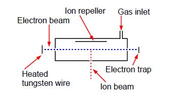
Above Figure shows a stainless steel source of a mass spectrometer which is inside a vacuum chamber at a pressure of about 10^-10 atm. A beam of electrons (from a heated tungsten filament) is passed through a low pressure of helium gas (~10^-7 atm.) and the probability of ionization, called the cross section S (in angstrom squared Å² =10^-20 m²) is measured as a function of the colliding electron’s energy, E, (measured in a unit called the electron volt, eV).

e_{KE1 +}He → e_KE2+He⁺ + e_KE3

The impacting electron losses kinetic energy in the collision from KE1 to KE2 and the energy lost is required to both ionize the helium atom and give the liberated slow electron its kinetic energy of KE3. Helium ionizes at E = 24.59 eV and then S increases to a broad plateau at E = 60-80 eV after which S decreases slowly with E. There are good theoretical reasons for believing that our high energy data, beyond the plateau region, should fit the equation,

S (E) = A – A exp (B/E)

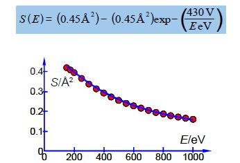
Where A and B are unknown coefficients. From the data in below Figure design a spreadsheet and use Solver to find the unknown coefficients and then plot the data with its NLLSQ line. Using your equation what is the cross section for ionization of helium with 485 eV electrons and what is the precision of this cross-section?

	A	B
1	E/eV	S/Å²
2	150	0.43
3	175	0.40
4	200	0.39
5	250	0.37
6	300	0.34
7	350	0.31
8	400	0.28
9	450	0.27
10	500	0.26
11	550	0.24
12	600	0.23
13	650	0.21
14	700	0.21
15	750	0.19
16	800	0.19
17	850	0.17
18	900	0.17
19	950	0.17
20	1000	0.16

Solution: Ionization of He

Below Fig. is the spreadsheet for the NLLSQ fitting of the ionization data for helium for our model equation.

	A	B	C	D	E	F
1	E/eV	S/Å²	S(calc)	SR
2	150	0.43	0.420136	0.000097	A =	0.446103
3	175	0.40	0.407121	0.000051	B =	426.554
4	200	0.39	0.393236	0.000010
5	250	0.37	0.365113	0.000024
6	300	0.34	0.338473	0.000002
7	350	0.31	0.314232	0.000018
8	400	0.28	0.292532	0.000157
9	450	0.27	0.273214	0.000010
10	500	0.26	0.256024	0.000016
11	550	0.24	0.240695	0.000000
12	600	0.23	0.226982	0.000009
13	650	0.21	0.214665	0.000022
14	700	0.21	0.203558	0.000041
15	750	0.19	0.193502	0.000012
16	800	0.19	0.184362	0.000032
17	850	0.17	0.176022	0.000036
18	900	0.17	0.168387	0.000003
19	950	0.17	0.161372	0.000074
20	1000	0.16	0.154907	0.000026
21
22			SSR =	0.000642

Column C is the calculated cross section S e.g. cell C2 is:

($F$2) – ($F$2 x exp (-$F$3/A2))

and the SR in D2 is = (B2-C2)². The formulae from C2 and D2 are copied down to C20 and D20 with the appropriate variable for column A. The SSR in cell D22 is =SUM(D2:D20).

The next important task is the initial guess for A and B. Entering the default A = 1 and B = 1 gives the sum of squares equals to 1.42. The first value for S is around 0.4 so A should be around 0.4. Trial and error by typing in various values for the constants with A = 0.4 and typing in B as 100, 200, 300, 400, 500 and 600 gives shows that B = 500 has SSR = 0.004 which is the smallest value. So the initial estimates are A = 0.4 and B = 500. Selecting DEPS and editing cycle limit to 2,000,000 and stagnation limit 70,000. Solver reaches stagnation after 17 seconds with 1096 iterations and SSR = 6.42×10^-4.

Altering the digits of each constant looking for changes of an order of magnitude in SSR gives the following model equation. The NLLSQ equation is shown below with the last significant figure shown A = 0.45 ± 0.01 Å² and with B = 430 ± 20 eV. Below Fig shows a graph of the experimental data with our fitted equation.