Unless the line is terminated with the characteristic impedance there will also be reflected waves traveling in the -x direction, and the wave amplitude will be the sum of incident and reflected components. If the line is open-circuit, i.e. nothing connected to output terminals, the resistance is infinite. In this case the reflected wave will be inverted and the result will be a standing wave. To see this let’s apply the boundary condition on the current, namely at the open circuited end the current must be zero as the charge cannot move in or out of the open-circuit end of the transmission line. If we set the open-circuit end of the transmission line to be at x = 0, then we must have
I (0, t) = If e-iωt + Ib e-iωt = 0.
This condition can only be met for all t if Ib = -If, i.e. total reflection with the reflected wave inverted. Fbr convenience, we can set Ib = I0 /2i, and then we have
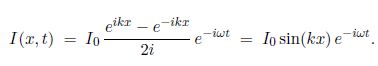
Taking the real part, we have a standing wave as in below Fig,
I (x, t) = I0 sin (kx) cos (wt).
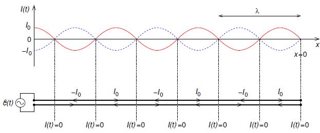
Figure: The current as a function of position along an open circuited lossless transmission line is a standing wave: red solid curve — current at t = nT where n is an integer and T = 2π/w is the period; blue dashed curve — current at t = (n + ½ )T. Note that curent nodes (where I = 0) occur at every half wavelength from the open-circuit end where x = 0; the wavelength is λ = 2π/k. The lower plot shows direction of current flow in each conductor at t = nT.