A protein has been complexed with a molecule to form a compound that absorbs in the UV-visible range of the spectrum. In the Chemistry lab we use a spectrophotometer, see Fig. 1.1, to measure the absorption of the light. White light from a radiation source is selected for the wavelength at which the complex has a strong absorption. The selected wavelength has an intensity 10 which is passed through a known concentration of the complex, c mol L^-1, and a known length of the sample, I cm.
The intensity of the light will be reduced by absorption of the complex to an intensity L The log(Io /I) is called the absorbance, A, of the solution and from the Beer-Lambert law, see below, the absorbance is proportional to the concentration of the absorbing molecule, c, the length of the sample, I, and the absorption coefficient of the molecule, e. The absorption coefficient of the molecule e varies with the wavelength of light and hence the need for using monochromatic light.

Figure: 1.1


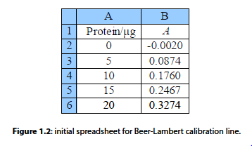
Fig. 1.2 is the initial spreadsheet of different known concentrations of the protein-complex and their absorbances. Fitting a line through the data points gives us a calibration curve for the complex. Obtaining the calibration curve means that we can measure an unknown concentration of the complex, e.g. obtained from a patient in a hospital.
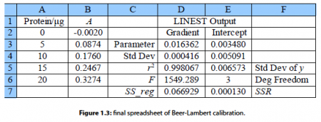
To use the function LINEST we firstly select a blank area of the spreadsheet of 2 columns by 5 rows, let’s assume this array of blank cells is D3 to E7. While this array of blank cells is still selected (high lighted) you enter your LINEST array-equation in the function window of the spreadsheet as,
LINEST (B2:B6, A2:A6, 1, 1)
These four parameters within LINEST have the following meanings. The cells B2:B6 are the y-data and the cells A2:A6 are the x-data. The third parameter is a switch; if for good chemical reasons you want the line to go through the origin (0, 0) then set this parameter to 0, otherwise to find the intercept set it to 1. The fourth parameter is also a switch, if it is set to 0 then only the gradient and intercept are calculated, we will set it to 1 to obtain all the other statistics as well. These four parameters are separated by commas. Do not click on the arrow next to the function window and do not press return as this LINEST formula is an array formula, the array is from A2 to E7, instead enter the array formula with shift-control-return on a PC or command-return on a Mac. The blank cells you selected will now fill up with the LLSQ fitted parameters as in Fig. 1.3.

Here typed labels into the spreadsheet in columns C and F to help us understand the statistics produced. In cell D3 is the gradient m and E3 the intercept c. D4 is the standard deviation of the gradient ai. and E4 the standard deviation of the intercept cc. D5 is the correlation coefficient r2 which for a good fit should be a number close to but less than unity. Of the other statistics, the ones of interest are E6 the number of degrees of freedom which is the number of data points, 5 in this example, minus the number of coefficients to be fitted, 2 for m and c, so in this example the number of degrees of freedom is 3. E7 is the minimized value of the SSR of the fitted line which has been minimized by the LINEST algorithm of the spreadsheet.
We quote the equation for our least squares line with the first decimal figure of the standard deviations (rounded if necessary) giving us the last decimal figure of the gradient and the intercept (also rounded if necessary). The LINEST fitted Beer-Lambert law calibration line is,
![]()
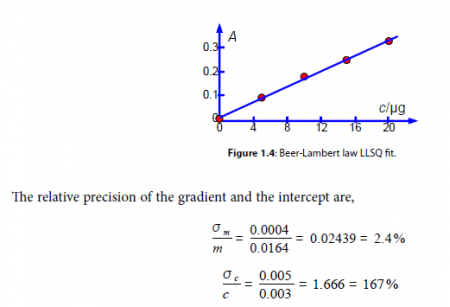
From our model equation (the Beer-Lambert law) the absorbance is dimensionless A = log(4 a ) and should pass through the origin. The graph of A against c is shown in Fig. 1.4 and the gradient m should have a gradient of units 1 /c or lir’. The intercept has the units of A and is dimensionless. A graph should always be plotted to check that no mistakes have been made and there is not a rogue data point that needs to be either measured again or not plotted as it distorts the data too much. The line shown in Fig. 1.4 is our LLSQ line from the LINEST spreadsheet.

Clearly interpolating within the range 0 to 20 ug of protein for the unknown sample is valid, but extrapolating for an amount of protein greater than 20 Kg should definitely not be attempted due to the large uncertainty in the intercept. Looking at the graph in Fig. 1.4 we might be tempted to try extrapolation but the size of the standard deviation of the intercept tells us that we would need to make experimental measurements at higher concentrations and not extrapolate the graph.


